Simulate from a model object

This function sets up the simulation run from data stored in the model object as well as arguments passed in. Use mrgsim_q() instead to benchmark mrgsolve or to do repeated quick simulation for tasks like parameter optimization, sensitivity analyses, or optimal design. See mrgsim_variants for other mrgsim-like functions that have more focused inputs. mrgsim_df coerces output to data.frame prior to returning.

Usage

mrgsim(x, data = NULL, idata = NULL, events = NULL, nid = NULL, ...)

mrgsim_df(..., output = "df")

do_mrgsim(
  x,
  data,
  idata = no_idata_set(),
  carry_out = carry.out,
  carry.out = character(0),
  recover = character(0),
  seed = as.integer(NA),
  Request = character(0),
  output = NULL,
  capture = NULL,
  obsonly = FALSE,
  obsaug = FALSE,
  tgrid = NULL,
  etasrc = "omega",
  recsort = 1,
  deslist = list(),
  descol = character(0),
  filbak = TRUE,
  tad = FALSE,
  nocb = TRUE,
  skip_init_calc = FALSE,
  ss_n = 500,
  ss_fixed = FALSE,
  interrupt = 256,
  ...
)

Arguments

x: the model object
data: NMTRAN-like data set (see data_set())
idata: a matrix or data frame of model parameters, one parameter per row (see idata_set())
events: an event object
nid: integer number of individuals to simulate; only used if idata and data are missing
...: passed to update() and do_mrgsim()
output: if NULL (the default) a mrgsims object is returned; otherwise, pass df to return a data.frame or matrix to return a matrix.
carry_out: numeric data items to copy into the output.
carry.out: soon to be deprecated; use carry_out instead.
recover: character column names in either data or idata to join back (recover) to simulated data; may be any class (e.g. numeric, character, factor, etc).
seed: deprecated.
Request: compartments or captured variables to retain in the simulated output; this is different than the request slot in the model object, which refers only to model compartments.
capture: character file name used for debugging (not related to $CAPTURE).
obsonly: if TRUE, dosing records are not included in the output.
obsaug: augment the data set with time grid observations; when TRUE and a full data set is used, the simulated output is augmented with an observation at each time in stime(). When using obsaug, a flag indicating augmented observations can be requested by including a.u.g in carry_out.
tgrid: a tgrid object; or a numeric vector of simulation times or another object with an stime method.
etasrc: source for ETA() values in the model; values can include: "omega", "data", "data.all", "idata", or "idata.all"; see 'Details'.
recsort: record sorting flag. Default value is 1. Possible values are 1,2,3,4: 1 and 2 put doses in a data set after padded observations at the same time; 3 and 4 put those doses before padded observations at the same time. 2 and 4 will put doses scheduled through addl after observations at the same time; 1 and 3 put doses scheduled through addl before observations at the same time. recsort will not change the order of your input data set if both doses and observations are given.
deslist: a list of tgrid objects.
descol: the name of a column for assigning designs.
filbak: carry data items backward when the first data set row has time greater than zero.
tad: when TRUE a column is added to simulated output is added showing the time since the last dose. Only data records with evid == 1 will be considered doses for the purposes of tad calculation. The tad can be properly calculated with a dosing lag time in the model as long as the dosing lag time (specified in $MAIN) is always appropriate for any subsequent doses scheduled through addl. This will always be true if the lag time doesn't change over time. But it might (possibly) not hold if the lag time changes prior to the last dose in the addl sequence. This known limitation shouldn't affect tad calculation in most common dosing lag time implementations.
nocb: if TRUE, use next observation carry backward method; otherwise, use locf.
skip_init_calc: don't use $MAIN to calculate initial conditions.
ss_n: maximum number of iterations for determining steady state for the PK system; a warning will be issued if steady state is not achieved within ss_n iterations when ss_fixed is TRUE.
ss_fixed: if FALSE (the default), then a warning will be issued if the system does not reach steady state within ss_n iterations given the model tolerances rtol and atol; if TRUE, the number of iterations for determining steady state are capped at ss_n and no warning will be issued if steady state has not been reached within ss_n dosing iterations. To silence warnings related to steady state, set ss_fixed to TRUE and set ss_n as the maximum number of iterations to try when advancing the system for steady state determination.
interrupt: integer check user interrupt interval; when interrupt is a positive integer, the simulation will check for the user interrupt signal every interrupt simulation records; pass a negative number to never check for the user interrupt interval.

Value

An object of class mrgsims

Details

Use mrgsim_df() to return a data frame rather than mrgsims object
Both data and idata will be coerced to numeric matrix
carry_out can be used to insert data columns into the output data set. This is partially dependent on the nature of the data brought into the problem
When using data and idata together, an error is generated if an ID occurs in data but not idata. Also, when looking up data in idata, ID in idata is assumed to be uniquely keyed to ID in data. No error is generated if ID is duplicated in data; parameters will be used from the first occurrence found in idata
carry_out: idata is assumed to be individual-level and variables that are carried from idata are repeated throughout the individual's simulated data. Variables carried from data are carried via last-observation carry forward. NA is returned from observations that are inserted into simulated output that occur prior to the first record in data
recover: this is similar to carry_out with respect to end result, but it uses a different process. Columns to be recovered are cached prior to running the simulation, and then joined back on to the simulated data. So, whereas carry_out will only accept numeric data items, recover can handle data frame columns of any type. There is a small decrease in performance with recover compared to carry_out, but it is likely that the performance difference is difficult to perceive (when the simulation runs very fast) or only a small fractional increase in run time when the simulation is very large. And any performance hit is likely to be well worth it in light of the convenience gain. Just think carefully about using this feature when every millisecond counts.
etasrc: this argument lets you control where ETA(n) come from in the model. When etasrc is set to "omega" (the default), ETAs will be simulated from a multivariate normal distribution defined by the $OMEGA blocks in the model. Alternatively, input data or idata sets can be used to pass in fixed ETA(n) by setting etasrc to "data", "idata", "data.all" or "idata.all". When etasrc is set to "data" or "data.all", the input data set will be scanned for columns called ETA1, ETA2, ..., ETAn and those values will be copied into the appropriate slot in the ETA() vector. Only the first record for each individual will be copied into ETA(); all records after the first will be ignored. When there are more than 9 ETAs in a model, NONMEM will start naming the outputs ET10, ET11 etc rather than ETA10 and ETA11. When mrgsolve is looking for these columns, it will first search, for example, ET10 and use that value if it is found. If ET10 isn't found and there are more than 9 ETAs, then it will also search for ETA10. An error will be generated in case mrgsolve finds both the ETA and ET name variant for the tenth and higher ETA (e.g. it is an error to have both ETA10 and ET10 in the data set). When mrgsolve is searching for ETA columns in the data set, it will only look for ETAn up to the number of rows (or columns) in all the model $OMEGA blocks. For example, if $OMEGA is 5x5, only ETA1 through ETA5 will be searched. An error will be generated in case mrgsolve finds no columns with ETAn names and something other than etasrc = "omega" was passed. When etasrc = "data" and an ETAn column is missing from the data set, the missing ETA() will be set to 0. Alternatively, the user can pass etasrc = "data.all" which causes an error to be generated if any ETAn is missing from the data set. Use this option when you intend to have all ETAs attached to the data set and want an error generated if mrgsolve finds one or more of them is missing. Using etasrc ="idata" or "idata.all", the behavior is identical to "data" (or "data.all"), except mrgsolve will look at the idata set rather than data set.

Examples

## example("mrgsim")

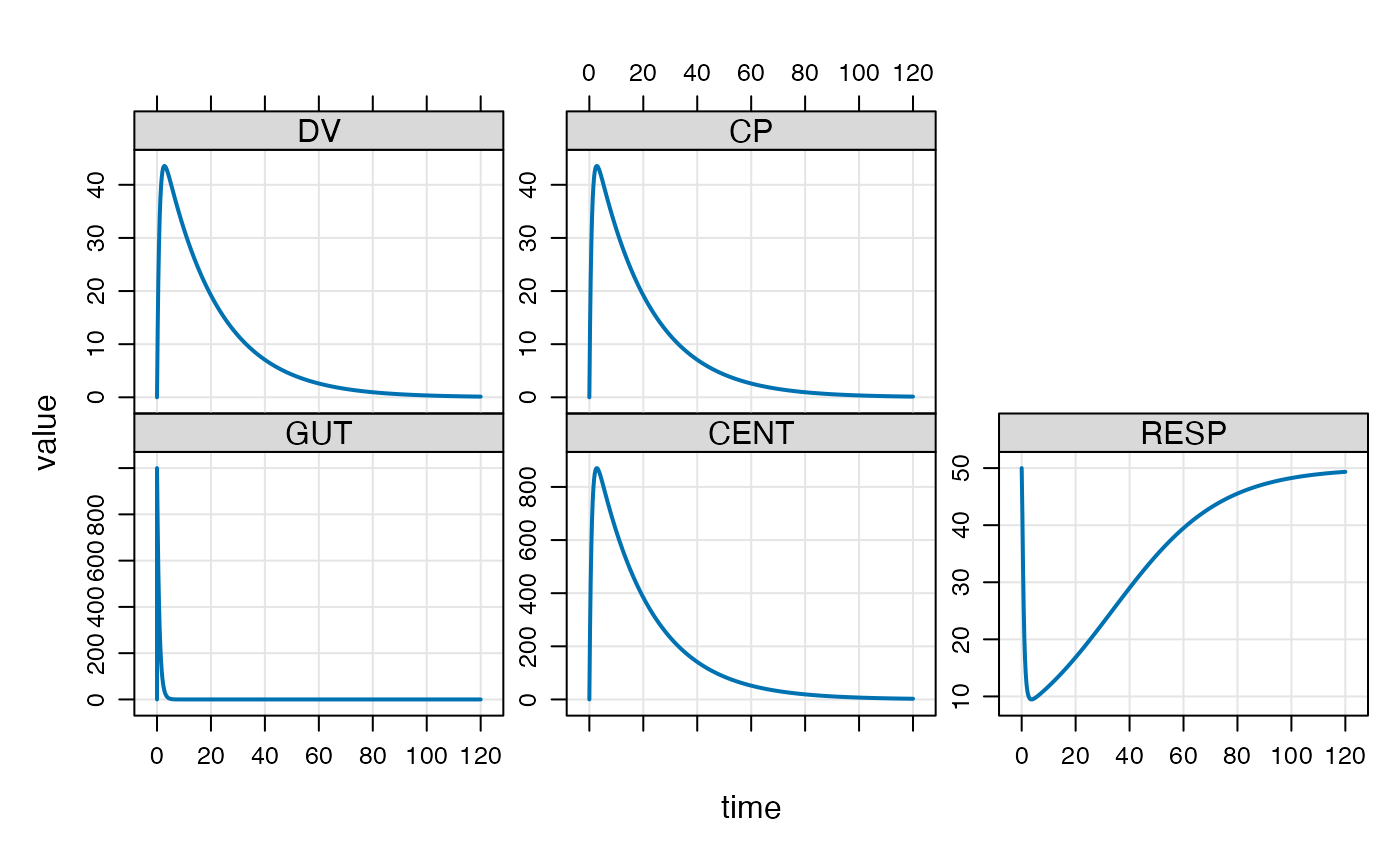
e <- ev(amt = 1000)

mod <- mrgsolve::house() 

out <- mod %>% ev(e) %>% mrgsim()

plot(out)


out <- mod %>% ev(e) %>% mrgsim(end=22)

out
#> Model:  housemodel 
#> Dim:    90 x 7 
#> Time:   0 to 22 
#> ID:     1 
#>     ID time    GUT  CENT  RESP    DV    CP
#> 1:   1 0.00    0.0   0.0 50.00  0.00  0.00
#> 2:   1 0.00 1000.0   0.0 50.00  0.00  0.00
#> 3:   1 0.25  740.8 257.5 42.29 12.87 12.87
#> 4:   1 0.50  548.8 445.0 32.69 22.25 22.25
#> 5:   1 0.75  406.6 580.8 25.29 29.04 29.04
#> 6:   1 1.00  301.2 678.3 20.05 33.91 33.91
#> 7:   1 1.25  223.1 747.4 16.45 37.37 37.37
#> 8:   1 1.50  165.3 795.6 14.01 39.78 39.78

data(exTheoph)

out <- mod %>% data_set(exTheoph) %>% mrgsim()

out
#> Model:  housemodel 
#> Dim:    132 x 7 
#> Time:   0 to 24.65 
#> ID:     12 
#>     ID time      GUT  CENT  RESP      DV      CP
#> 1:   1 0.00 4.020000 0.000 50.00 0.00000 0.00000
#> 2:   1 0.25 2.978089 1.035 49.95 0.04552 0.04552
#> 3:   1 0.57 2.028470 1.961 49.81 0.08624 0.08624
#> 4:   1 1.12 1.048417 2.875 49.57 0.12643 0.12643
#> 5:   1 2.02 0.356038 3.428 49.33 0.15072 0.15072
#> 6:   1 3.82 0.041060 3.439 49.25 0.15121 0.15121
#> 7:   1 5.10 0.008838 3.263 49.28 0.14348 0.14348
#> 8:   1 7.03 0.000872 2.980 49.34 0.13101 0.13101

out <- mod %>% mrgsim(data=exTheoph)

out <- mrgsim(mod, data=exTheoph, obsonly=TRUE)

out
#> Model:  housemodel 
#> Dim:    120 x 7 
#> Time:   0.25 to 24.65 
#> ID:     12 
#>     ID time       GUT  CENT  RESP      DV      CP
#> 1:   1 0.25 2.978e+00 1.035 49.95 0.04552 0.04552
#> 2:   1 0.57 2.028e+00 1.961 49.81 0.08624 0.08624
#> 3:   1 1.12 1.048e+00 2.875 49.57 0.12643 0.12643
#> 4:   1 2.02 3.560e-01 3.428 49.33 0.15072 0.15072
#> 5:   1 3.82 4.106e-02 3.439 49.25 0.15121 0.15121
#> 6:   1 5.10 8.838e-03 3.263 49.28 0.14348 0.14348
#> 7:   1 7.03 8.720e-04 2.980 49.34 0.13101 0.13101
#> 8:   1 9.05 7.723e-05 2.703 49.40 0.11884 0.11884

out <- mod %>% mrgsim(data=exTheoph, obsaug=TRUE, carry_out="a.u.g")

out
#> Model:  housemodel 
#> Dim:    5904 x 8 
#> Time:   0 to 120 
#> ID:     12 
#>     ID time a.u.g   GUT  CENT  RESP      DV      CP
#> 1:   1 0.00     1 0.000 0.000 50.00 0.00000 0.00000
#> 2:   1 0.00     0 4.020 0.000 50.00 0.00000 0.00000
#> 3:   1 0.25     1 2.978 1.035 49.95 0.04552 0.04552
#> 4:   1 0.25     0 2.978 1.035 49.95 0.04552 0.04552
#> 5:   1 0.50     1 2.206 1.790 49.84 0.07870 0.07870
#> 6:   1 0.57     0 2.028 1.961 49.81 0.08624 0.08624
#> 7:   1 0.75     1 1.634 2.337 49.73 0.10274 0.10274
#> 8:   1 1.00     1 1.211 2.729 49.61 0.12001 0.12001

out <- mod %>% ev(e) %>% mrgsim(outvars="CP,RESP")

out
#> Model:  housemodel 
#> Dim:    482 x 4 
#> Time:   0 to 120 
#> ID:     1 
#>     ID time  RESP    CP
#> 1:   1 0.00 50.00  0.00
#> 2:   1 0.00 50.00  0.00
#> 3:   1 0.25 42.29 12.87
#> 4:   1 0.50 32.69 22.25
#> 5:   1 0.75 25.29 29.04
#> 6:   1 1.00 20.05 33.91
#> 7:   1 1.25 16.45 37.37
#> 8:   1 1.50 14.01 39.78

a <- ev(amt = 1000, group = 'a')
b <- ev(amt = 750, group = 'b')
data <- as_data_set(a,b)

out <- mrgsim_d(mod, data, recover="group")

out
#> Model:  housemodel 
#> Dim:    964 x 8 
#> Time:   0 to 120 
#> ID:     2 
#>     ID time    GUT  CENT  RESP    DV    CP group
#> 1:   1 0.00    0.0   0.0 50.00  0.00  0.00     a
#> 2:   1 0.00 1000.0   0.0 50.00  0.00  0.00     a
#> 3:   1 0.25  740.8 257.5 42.29 12.87 12.87     a
#> 4:   1 0.50  548.8 445.0 32.69 22.25 22.25     a
#> 5:   1 0.75  406.6 580.8 25.29 29.04 29.04     a
#> 6:   1 1.00  301.2 678.3 20.05 33.91 33.91     a
#> 7:   1 1.25  223.1 747.4 16.45 37.37 37.37     a
#> 8:   1 1.50  165.3 795.6 14.01 39.78 39.78     a

Usage

Arguments

Value

Details

See also

Examples