Quick hit demos
These are all miscellaneous features that may be difficult to find in other documentation.
$ operator for model object gets the parameter value
If our model parameters are
 Model parameters (N=14):
 name value . name  value
 CL   1     | SEX   0
 D1   2     | SEXCL 0.7
 F1   1     | SEXVC 0.85
 IC50 10    | VC    20
 KA   1.2   | WT    70
 KIN  100   | WTCL  0.75
 KOUT 2     | WTVC  1
we can pick a parameter value with
Or slice off multiple parameters
Model names
For programming with a model object, we can extract the names
$param
 [1] "CL"    "VC"    "KA"    "F1"    "D1"    "WTCL"  "WTVC"  "SEXCL" "SEXVC"
[10] "KIN"   "KOUT"  "IC50"  "WT"    "SEX"

$init
[1] "GUT"  "CENT" "RESP"

$capture
[1] "DV" "CP"

$omega
[1] "..."

$sigma
[1] "..."

$omega_labels
$omega_labels[[1]]
[1] "ECL"   "EVC"   "EKA"   "EKOUT"


$sigma_labels
$sigma_labels[[1]]
[1] "EXPO"
or get all of the model elements in a list (output not shown)
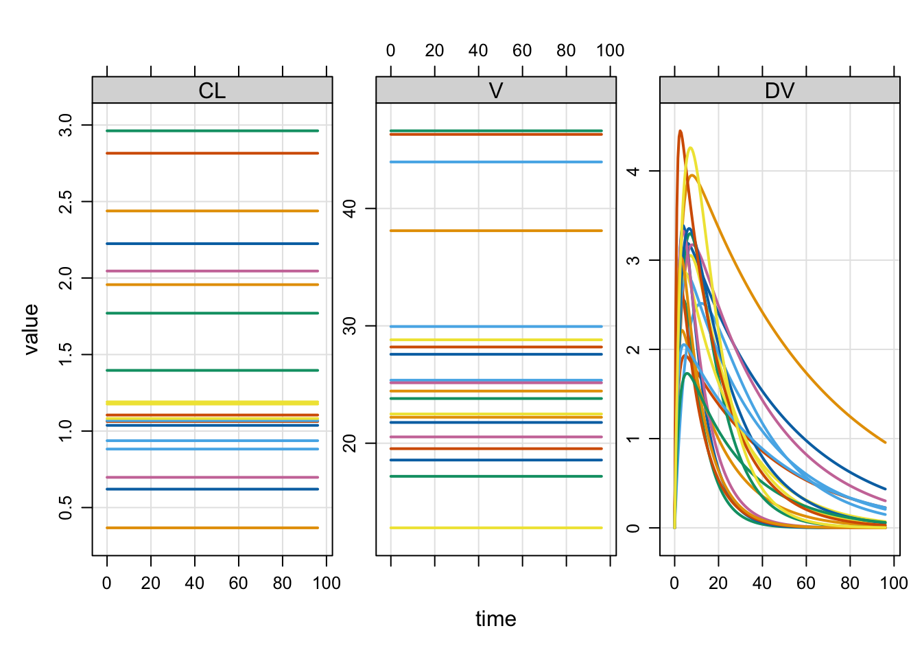
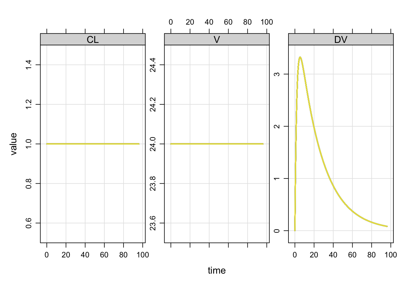
Zero all random effect variances on the fly
If your model has random effects, you can easily and temporarily zero them out.
Building popex ... done.$...
[,1] [,2] [,3]
ECL: 0.3 0.0 0.0
EV: 0.0 0.1 0.0
EKA: 0.0 0.0 0.5It is easy to simulate either with or without the random effects in the simulation: this change can be made on the fly.
Use zero_re to make all random effect variances zero
By default, both OMEGA and SIGMA are zeroed. Check the arguments for zero_re to see how to selectively zero OMEGA or SIGMA.
Compare the population output
with
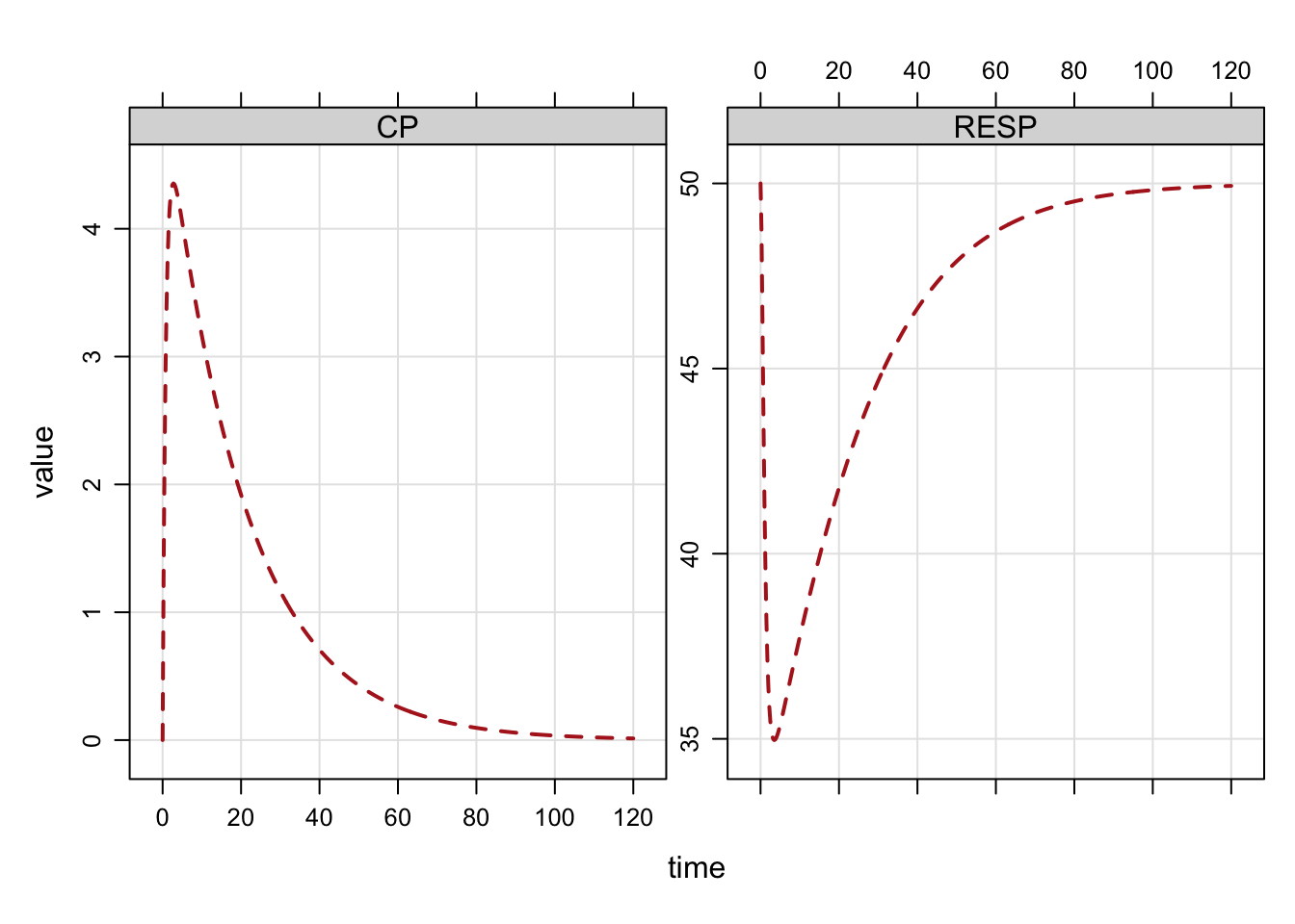
Plot formulae
We commonly plot simulated output with a special plot method. By default, you get all compartments and output variables in the plot.
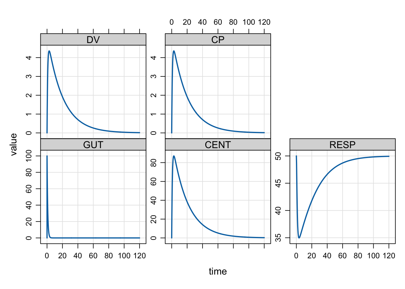
The plot can be customized with a formula selecting variables to plot. Other arguments
to lattice::xyplot can be passed as well.
Get a data frame of simulated data
By default mrgsolve returns an object of simulated data (and other stuff)
But you can get a data frame with
or